1. INTRODUCTION
Population structure and genetic diversity analyses are important ways to find out the genetic relationship and evolutionary history among the species. Studies on population structure and genetic diversity provide a framework to explore the ecological and conservation issues for species management. Details of population structure and genetic diversity are essential and invaluable to understanding the gene flow, genetic drift, and natural selection processes among populations [1]. Molecular markers are useful for assessing the genetic variation within and among species. Random Amplified Polymorphic DNA (RAPD) markers are dominant DNA markers and were commonly used to study population structure and genetic diversity [2,3].
Dalbergia latifolia Roxb. and Dalbergia sissoides Wight and Arn. are valuable and precious timber species of the family Fabaceae. D. latifolia is known as “Indian Rosewood” or “Bombay Blackwood” and distributed in the sub-Himalayan tract from Oudh eastwards to Sikkim, Bihar, Orissa, Central, Western, and Southern India. D. sissoides is commonly known as “Malabar Blackwood” and distributed in Western Ghats of Karnataka, Tamil Nadu, and Kerala. These tree species are found in the semi-evergreen and deciduous forests of the above areas. The timber of these species was used for making furniture, carvings, decorative plywood, and veneers [4,5].
D. latifolia and D. sissoides are genetically closer species and have a wide range of habitat-preferring morphological characteristics which caused many difficulties in species identification using herbarium specimens [6]. Therefore, earlier taxonomical studies considered D. sissoides as a variety of D. latifolia and mentioned it as D. latifolia var. sissoides (Wight and Arn.) Baker whereas, later studies separated it as a distinct species [7,8]. Hiremath and Nagasampige (2004) showed a high jaccard similarity index (0.37) between these species was noted using RAPD markers in the Western Ghats of Karnataka and supports the independent species status of D. sissoides [9]. Yulita et al. reported the genetic diversity of five populations of D. latifolia from Yogyakarta and Lombok Island, West Nusa Tenggara, Indonesia, using sequence random amplified polymorphism (SRAP) markers [10]. Yulita et al. also revealed the population structure and genetic diversity study of D. latifolia in Java and West Nusa Tenggara using SRAP markers [11].
Many natural factors and illegal logging have affected the reproduction and establishment of these tree species. Therefore, the natural populations of these species have been declining in their habitats [5]. Both rosewood species were listed in Appendix 2 of CITES since 2017. The species appearing in Appendix 2 of CITES were banned from international trade without an import and export license or re-export certificate [10]. Both rosewood species have also been categorized as “Vulnerable” in the Red Data Book of IUCN [13]. Hence, population structure and genetic diversity studies of these species are essential for developing conservation strategies and further tree improvement programs.
2. MATERIALS AND METHODS
2.1. Establishing of Germplasm Assemblage
Field surveys were undertaken in Gudalur, Coimbatore, Erode, Salem, Dharmapuri, Theni, Tirunelveli forest divisions of Tamil Nadu and Kannur, Wayanad, Nilambur, Mannarkad, Palakkad, Chalakkudy, Nemmara, Malayattor, Munnar, Ranni, Konni, and Thiruvanandapuram forest divisions of Kerala and altogether 173 morphologically superior D. latifolia and D. sissoides trees were selected. The species were differentiated mainly based on the morphological characters of leaflets [Figure 1]. However, many trees showed a wide range of variations in leaflet morphology which makes them very difficult to classify. The root cuttings were collected from the selected trees, vegetatively propagated and used to establish the clonal germplasm assemblage [14]. Dalbergia clones (56 Nos) from the above assemblage were used for the present study and listed in Table 1. Indian Rosewood seedlings (KFRI-1 and KFRI-2) bought from Kerala Forest Research Institute, Peechi were used as check or control trees for D. latifolia.
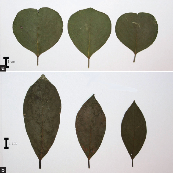 | Figure 1: Leaflets of Dalbergia latifolia and Dalbergia sissoides. (a) D. latifolia leaflets with retuse and obtuse apex. (b) D. sissoides leaflets with acute apex. [Click here to view] |
Table 1: Geographical locations of Dalbergia latifolia and Dalbergia sissoides populations in Kerala and Tamil Nadu.
| S. No. | Clone name | Forest Range | Forest division/population | Region/state | Latitude | Longitude | Elevation (masl) |
|---|---|---|---|---|---|---|---|
| 1 | KLPKWAL-1 | Walayar | Palakkad | Kerala | 10° 51’20.6” | 76° 48’ 34.0” | 360.4 |
| 2 | KLPKWAL-5 | Walayar | Palakkad | Kerala | 10° 49’ 49.4” | 76° 47’ 43.6” | 360.3 |
| 3 | KLNMNEL-1 | Nelliyampathy | Nemmara | Kerala | 10° 26’ 44” | 76° 42’ 35” | 353.7 |
| 4 | KLNMNEL-3 | Nelliyampathy | Nemmara | Kerala | 10° 31’ 16” | 76° 37’ 51” | 329.4 |
| 5 | KLNMNEL-6 | Nelliyampathy | Nemmara | Kerala | 10° 31’ 39” | 76° 37’ 47” | 326.8 |
| 6 | KLNMNEL-8 | Nelliyampathy | Nemmara | Kerala | 10° 31’ 38” | 76° 37’ 46” | 326.8 |
| 7 | KLCHPAL-1 | Palappally | Chalakudy | Kerala | 10° 26’ 21” | 76° 23’ 28” | 211.9 |
| 8 | KLCHPAL-6 | Palappally | Chalakudy | Kerala | 10° 26’ 27” | 76° 23’ 51” | 213.2 |
| 9 | KLCHVEL-2 | Vellikulangara | Chalakudy | Kerala | 10° 23’ 10” | 76° 24’ 22” | 221.3 |
| 10 | KLCHVEL-5 | Vellikulangara | Chalakudy | Kerala | 10° 22’ 54” | 76° 24’ 42” | 224.3 |
| 11 | KLMKAGL-4 | Agali | Mannarkad | Kerala | 11° 02’ 02.2” | 76° 37’ 56.8” | 289.1 |
| 12 | KLMKATP-1 | Attappady | Mannarkad | Kerala | 11° 09’ 59.2” | 76° 38’ 26.0” | 271.3 |
| 13 | KLMYKUT-1 | Kuttampuzha | Malayattoor | Kerala | 10° 10’ 33.9” | 76° 47’ 04.7” | 462.5 |
| 14 | KLMYKUT-3 | Kuttampuzha | Malayattoor | Kerala | 10° 09’ 27” | 76° 46’ 13” | 458.8 |
| 15 | KLMYKUT-7 | Kuttampuzha | Malayattoor | Kerala | 10° 09’ 26” | 76° 45’ 35” | 458.8 |
| 16 | KLKNKAN-1 | Kannavam | Kannur | Kerala | 11° 47’ 46.9” | 75° 44’ 29.8” | 395.1 |
| 17 | KLKNKAN-5 | Kannavam | Kannur | Kerala | 11° 47’ 46.9” | 75° 44’ 29.8” | 395.1 |
| 18 | KLKNTAL-2 | Thaliparamba | Kannur | Kerala | 12° 16’ 03.0” | 75° 26’ 06.0” | 375.7 |
| 19 | KLKNTAL-3 | Thaliparamba | Kannur | Kerala | 12° 16’ 03.0” | 75° 26’ 06.0” | 375.7 |
| 20 | KLMUADI-2 | Adimali | Munnar | Kerala | 10° 00’ 56.4” | 76° 54’ 01” | 570.9 |
| 21 | KLMUADI-3 | Adimali | Munnar | Kerala | 10° 00’ 55.3” | 76° 53’ 58.4” | 570.9 |
| 22 | KLMUNER-2 | Neriyamangalam | Munnar | Kerala | 10° 05’ 59.9” | 76° 51’ 00.8” | 513.0 |
| 23 | KLMUNER-4 | Neriyamangalam | Munnar | Kerala | 10° 05’ 01.9” | 76° 51’ 03.0” | 513.0 |
| 24 | KFRI-1 | KFRI | Thrissur | Kerala | - | - | - |
| 25 | KFRI-2 | KFRI | Thrissur | Kerala | - | - | - |
| 26 | KLTMPLO-4 | Palode | Thiruvanantha-puram | Kerala | 8° 42’ 16.1” | 77° 06’ 41.8” | 46.3 |
| 27 | KLTMPLO-5 | Palode | Thiruvanantha-puram | Kerala | 8° 42’ 16” | 77° 06’ 41.4” | 46.3 |
| 28 | KLKOKON-1 | Konni | Konni | Kerala | 9° 13’ 54.1” | 76° 54’ 54.3” | 205.7 |
| 29 | KLRAVAD-2 | Vadasserikkara | Ranni | Kerala | 9° 17’ 41.5” | 76° 57’ 27.9” | 243.7 |
| 30 | KLRAVAD-5 | Vadasserikkara | Ranni | Kerala | 9° 17’ 38.2” | 76° 57’ 31.5” | 243.2 |
| 31 | KLNLKAR-2 | Karulai | Nilambur | Kerala | 11° 16’ 36.7” | 76° 19’ 23.8” | 339.8 |
| 32 | KLNLKAR-4 | Karulai | Nilambur | Kerala | 11° 16’ 24.9” | 76° 21’ 52.9” | 344.3 |
| 33 | KLSWMEP-4 | Meppadi | Wayanad | Kerala | 11° 33’ 46.5” | 76° 04’ 22” | 509.2 |
| 34 | KLSWMEP-7 | Meppadi | Wayanad | Kerala | 11° 33’ 36.6” | 76° 04’ 09.3” | 508.7 |
| 35 | KLNWBEG-3 | Begur | Wayanad | Kerala | 11° 52’ 20” | 76° 03’ 24” | 740.7 |
| 36 | KLNWBEG-7 | Begur | Wayanad | Kerala | 11° 52’ 18.4” | 76° 03’ 29” | 740.6 |
| 37 | KLNWBEG-10 | Begur | Wayanad | Kerala | 11° 52’ 17.2” | 76° 03’ 28.8” | 740.6 |
| 38 | TNCBBOL-1 | Boluvampatty | Coimbatore | Tamil Nadu | 10° 56’ 28.2” | 76° 42’ 24.1” | 307.7 |
| 39 | TNCBBOL-4 | Boluvampatty | Coimbatore | Tamil Nadu | 10° 56’ 28.2” | 76° 42’ 24.1” | 307.7 |
| 40 | TNCBBOL-6 | Boluvampatty | Coimbatore | Tamil Nadu | 10° 57’ 45.4” | 76° 40’53.8” | 295.4 |
| 41 | TNEDBAR-2 | Bargur | Erode | Tamil Nadu | 11° 50’ 55” | 77° 34’ 26” | 507.2 |
| 42 | TNEDBAR-6 | Bargur | Erode | Tamil Nadu | 11° 48’ 55” | 77° 33’ 6” | 507.2 |
| 43 | TNEDBAR-8 | Bargur | Erode | Tamil Nadu | 11° 48’ 15” | 77° 32’ 55” | 517.8 |
| 44 | TNEDBAR-11 | Bargur | Erode | Tamil Nadu | 11° 51’ 17” | 77° 31’ 01” | 517.8 |
| 45 | TNTHCUM-1 | Cumbum | Theni | Tamil Nadu | 9° 37’ 24” | 77° 11’ 33” | 374.3 |
| 46 | TNTHCUM-6 | Cumbum | Theni | Tamil Nadu | 9° 37’ 18” | 77° 11’ 35” | 374.0 |
| 47 | TNDHHAR-4 | Harur | Dharmapuri | Tamil Nadu | 11° 51’ 57” | 78° 27’ 37.4” | 285.3 |
| 48 | TNDHHAR-8 | Harur | Dharmapuri | Tamil Nadu | 11° 51’ 51.5” | 78° 27’ 28.7” | 285.3 |
| 49 | TNSLSER-1 | Shervarayan | Salem | Tamil Nadu | 11° 46’ 16.3” | 78° 11’ 20.6” | 338.9 |
| 50 | TNSLYER-2 | Yercaud | Salem | Tamil Nadu | 11° 49’ 49.1” | 78° 16’ 46.2” | 328.3 |
| 51 | TNSLYER-3 | Yercaud | Salem | Tamil Nadu | 11° 49’ 56.8” | 78° 16’ 51.6” | 328.3 |
| 52 | TNSLDAN-2 | Danishpet | Salem | Tamil Nadu | 11° 50’ 28.6” | 78° 10’ 00.3” | 337.4 |
| 53 | TNTVCOR-2 | Courtallam | Tirunelveli | Tamil Nadu | 8° 55’ 38.1” | 77° 16’ 04.6” | 74.2 |
| 54 | TNTVCOR-10 | Courtallam | Tirunelveli | Tamil Nadu | 8° 55’ 55.0” | 77° 16’ 00.2” | 74.6 |
| 55 | TNGDCHR-3 | Cherambady | Gudalur | Tamil Nadu | 11° 35’ 03.0” | 76° 21’ 42.7” | 492.3 |
| 56 | TNGDBIT-10 | Bitherkad | Gudalur | Tamil Nadu | 11° 31’ 28.4” | 76° 16’ 33.0” | 534.4 |
KFRI-1 and KFRI-2 are Dalbergia latifolia seedlings bought from Kerala Forest Research Institute, Peechi, Thrissur.
2.2. Extraction and Purification of Genomic DNA
The young leaves of 56 D. latifolia and D. sissoides samples [Table 1] were collected from the germplasm assemblage and used for genomic DNA extraction following the CTAB method developed by Ginwal and Maurya with some modifications [15]. The extracted DNA samples were purified by RNase treatment (0.5 μg of RNase A used for 1 μg of DNA). The purified DNA was quantified using a spectrophotometer (NanoDrop™ Lite, Thermo Scientific). The quality of DNA ranged between 1.75 to 1.96 (A260/A280 value). The quantity of DNA ranged from 143 to 457 ng/μL. However, all samples were diluted to 50 ng/μL. The purified DNA samples were stored in a freezer at −20°C and used as template DNA in thermal cycler reactions.
2.3. Polymerase Chain Reaction and Gel Documentation
Each reaction mixture (15 μL of final volume) consisted of 7.5 μL of sterile water, 1.5 μL of 10X Taq buffer, 1.5 μL of 25 mM MgCl2, 1.5 μL of 10 mM dNTPs, 1.5 μL of 10 μM of RAPD Primer, 0.5 μL of Taq DNA polymerase (3U/μL), and 1 μL of template DNA. A thermal cycler (BIO-RAD T100™) was set up for DNA amplification according to the program with an initial denaturation at 94°C for 1 min, 40 cycles of denaturation at 94°C for 20 s, annealing at optimized temperature for 1 min, extension at 72°C for 2 min, then final extension at 72°C for 5 min and infinite hold at 12°C.
After completion of the above steps, the amplified PCR products were measured for their success through horizontal electrophoresis of 1.5% agarose gel mixed with ethidium bromide (0.5 μg/mL). The electrophoresis was carried out with 80 Voltage power for 3 h. The gel was documented using BIO-RAD Gel Doc™ XR+ Gel documentation system. The base pairs length of each band was estimated using Image Lab™ software (version 5.2.1).
2.4. Selection of High Polymorphic RAPD Markers
The randomly selected DNA of D. latifolia sample (TNCBBOL-1) was used to find out the best annealing temperature (Ta). The melting temperature (Tm) of RAPD primers ranged from 31.1 to 39.1°C. Therefore, RAPD markers were tested with different annealing temperatures viz., 27, 31, 35, 39, and 43°C. The amplified products of different annealing temperatures were run in agarose gel and documented. The best and most suitable annealing temperature was determined based on the band clearness [16].
The extracted DNA of nine randomly selected clones (KLNMNEL-1, TNCBBOL-1, KLNWBEG-10, TNSLSHR-1, TNEDBAR-11, KLKNTAL-2, KLPKWAL-1, TNTVCOR-2, and TNGDCHR-3) was used to select the high polymorphic RAPD primers. A total of 19 primers were tested with their respective optimized annealing temperatures. The high polymorphic primers were selected based on the high percentage of polymorphic bands.
2.5. Preparation of Binary or Dominant Marker Data
Each high polymorphic RAPD marker was separately amplified with 56 Dalbergia samples and the amplified products of eight RAPD markers were run in agarose gel and then digitally imaged [Figure 2]. The binary data were manually scored for the presence and absence of bands with 1 and 0, respectively, according to band size.
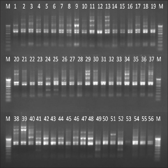 | Figure 2: A gel image of the RAPD 12 marker with 56 accessions of Dalbergia latifolia and Dalbergia sissoides. M – 100 bp DNA ladder, the numbers adherent at the top of each lane were represented the serial numbers of Table 1. [Click here to view] |
2.6. Estimation of Discriminatory Power of Selected RAPD Markers
The binary data were used to calculate the discriminatory power of selected RAPD markers [Table 2]. Genotypic gene diversity or expected heterozygosity, polymorphic information content, and effective multiplex ratio were computed using the formulas described by Sornakili et al., Chesnokov and Artemyeva, and Ismail et al., respectively [17-19]. Marker index and resolving power were calculated by using the formulas described by Dobhal et al., in Table 2 [20]. The relationships between the above parameters were calculated by the Pearson correlation coefficient method using IBM Statistical Package for the Social Sciences software (version 20).
Table 2: Discriminatory powers of selected RAPD markers are used in the present study.
| S. No. | Marker name | Sequence (5’ to 3’) | TNB | MB | PB | ABS (bp) | PPB | Hg | PIC | EMR | MI | RP |
|---|---|---|---|---|---|---|---|---|---|---|---|---|
| 1 | RAPD 1 | GGGAATTCGG | 12 | 1 | 11 | 210–3100 | 91.66 | 0.23 | 0.28 | 10.12 | 2.83 | 0.82 |
| 2 | RAPD 4 | CTGCTGGGAC | 12 | 0 | 12 | 226–2478 | 100 | 0.17 | 0.18 | 12 | 2.16 | 0.55 |
| 3 | RAPD 12 | GTGACGTAGG | 17 | 2 | 15 | 200–3850 | 88.23 | 0.13 | 0.18 | 13.2 | 2.38 | 0.53 |
| 4 | RAPD 13 | GGGTAACGCC | 12 | 1 | 11 | 320–1850 | 91.66 | 0.14 | 0.21 | 10.12 | 2.13 | 0.47 |
| 5 | RAPD 14 | TCGGCGATAG | 14 | 0 | 14 | 200–1780 | 100 | 0.18 | 0.23 | 14 | 3.22 | 0.49 |
| 6 | RAPD 15 | TCTGTGCTGG | 15 | 0 | 15 | 260–2048 | 100 | 0.2 | 0.23 | 15 | 3.45 | 0.52 |
| 7 | RAPD 16 | AGCCAGCGAA | 14 | 0 | 14 | 230–1754 | 100 | 0.18 | 0.22 | 14 | 3.08 | 0.43 |
| 8 | RAPD 17 | GAC CGCTTGT | 17 | 0 | 17 | 320–1950 | 100 | 0.13 | 0.19 | 17 | 3.23 | 0.31 |
| Total | 113 | 4 | 109 | 1.36 | 1.72 | 105.44 | 22.48 | 4.12 | ||||
| Average | 14.1 | 0.5 | 13.6 | 96.44 | 0.17 | 0.22 | 13.18 | 2.81 | 0.52 |
TNB: Total number of bands, MB: Monomorphic bands, PB: Polymorphic bands, ABS: Amplicon band size, PPB: Percentage of polymorphic band, Hg: Genotypic gene diversity or expected heterozygosity, PIC: Polymorphic information content, EMR: Effective multiplex ratio, MI: Marker index, RP: Resolving power.
2.7. Statistical Analysis
The RAPD data were also used for population structure and genetic diversity analysis. Population structure analysis was used to detect the subsets (number of K groups) of the whole sample by detecting allele frequency differences and to assign individuals in respective K groups based on the analysis of likelihoods. This analysis was performed with STRUCTURE software (version 2.3.4) using the Bayesian model and a web-based program STRUCTURE HARVESTER using the Evanno method [21,22]. In Evanno plot, the K group showed the highest Delta K value detected as the best fit for the dataset [Figure 3]. The population structure chart was derived based on the best-fitted K group [Figure 4]. The population structure map [Figure 5] was created using QGIS software (version 3.16.15).
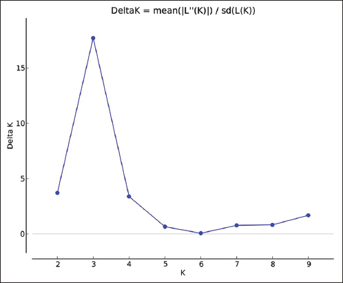 | Figure 3: Evanno plot with cluster numbers (k) in X axis and delta K values in Y axis. Cluster numbers 3 (K = 3) showed the high value of delta K (delta K =17.07) than other cluster numbers. [Click here to view] |
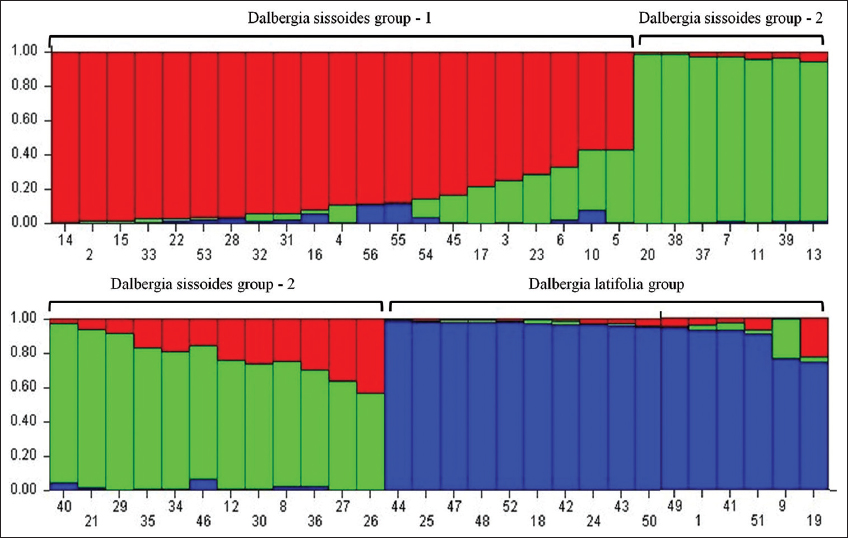 | Figure 4: The population structure chart showed 56 Dalbergia individuals which were categorized into 3 genotypic groups (Dalbergia sissoides group-1, 2 and Dalbergia latifolia group). The numbers in X axis were similar to the serial numbers of Table 1. [Click here to view] |
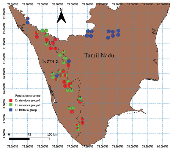 | Figure 5: Population structure map of Dalbergia sissoides and Dalbergia latifolia in Kerala and Tamil Nadu of India. [Click here to view] |
Principal coordinates analysis was a statistical method that converts RAPD data into distances between individuals and showed a map-based visualization of individuals [Figure 6]. This analysis was carried out with PAST software (version 4.03) using the Jaccard similarity coefficient [23].
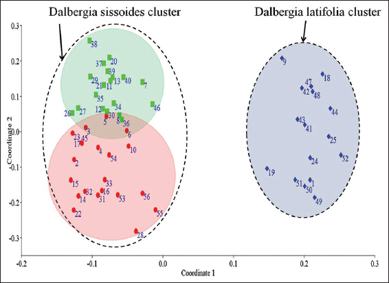 | Figure 6: Principal coordinates analysis showed Dalbergia latifolia and Dalbergia sissoides clusters. Blue diamond points – D. latifolia individuals, Red dot points – D. sissoides Group-1 individuals and Green square points – D. sissoides Group-2 individuals. The numbers adherent to each points were represented the serial numbers of Table 1. [Click here to view] |
Neighbor joining cluster analysis was a statistical method used to group an individual with other closely related individuals producing a dendrogram or phylogenetic tree as an outcome [Figure 7]. This analysis was performed by DAR win software (version 6.0.021) with unweighted neighbor joining method using the Jaccard dissimilarity coefficient along with 100 times bootstrapping [24].
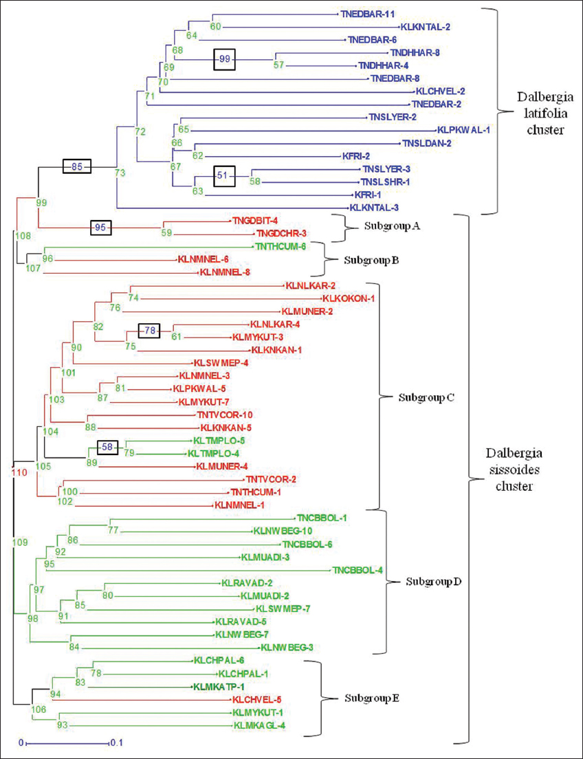 | Figure 7: Dendrogram of Dalbergia latifolia and Dalbergia sissoides using Unweighted Neighbour Joining method with Jaccard dissimilarity coefficient supported by ≥50% bootstrap values (box in the middle of branches) and node numbers. Blue - D. latifolia individuals, Red - D. sissoides group-1 individuals, Green - D. sissoides group-2 individuals. [Click here to view] |
Analysis of molecular variance (AMOVA) was a nonparametric analog method to detect molecular variance among individuals. AMOVA was performed based on Phi (π) statistics with 1000 permutations [Table 3]. Allele or gene frequency was the relative frequency of an allele at a particular locus in a population. It was used to find the genetic diversity among and within the populations. Genetic diversity within populations was estimated as Shannon information index, unbiased heterozygosity, and percentage of polymorphic loci [Tables 4 and 5]. Genetic diversity among populations was estimated as Nei’s genetic distance and genetic identity [Tables 6 and 7]. Similarly, genetic diversity between these species was estimated as Nei’s genetic distance and genetic identity. AMOVA and Allele frequency analysis were performed using GenAlEx software (version 6.502) [25].
Table 3: AMOVA of Dalbergia latifolia and Dalbergia sissoides from Kerala and Tamil Nadu.
| Species | Source | df | SS | MS | Est. Var. | PMV (%) | Stat | Value | P |
|---|---|---|---|---|---|---|---|---|---|
| Dalbergia latifolia | Among Kerala and Tamil Nadu | 1 | 11.783 | 11.783 | 0.000 | 0 | PhiRT | -0.045 | 0.903 |
| Among forest divisions | 4 | 62.217 | 15.554 | 2.396 | 20 | PhiPR | 0.204 | 0.001 | |
| Within forest divisions | 10 | 93.250 | 9.325 | 9.325 | 80 | PhiPT | 0.169 | 0.003 | |
| Total | 15 | 167.250 | 11.721 | 100 | |||||
| Dalbergia sissoides | Among Kerala and Tamil Nadu | 1 | 19.378 | 19.378 | 0.604 | 6 | PhiRT | 0.061 | 0.004 |
| Among forest divisions | 12 | 135.180 | 11.265 | 1.090 | 11 | PhiPR | 0.118 | 0.002 | |
| Within forest divisions | 26 | 211.967 | 8.153 | 8.153 | 83 | PhiPT | 0.172 | 0.001 | |
| Total | 39 | 366.525 | 9.846 | 100 |
df: Degree of freedom, SS: Sum of squared observations, MS: Mean of squared observations, Est. Var.: Estimated variance, PMV: Percentage of molecular variance, PhiRT: Proportion of the total genetic variance between the Kerala and Tamil Nadu regions, PhiPR: Proportion of the total genetic variance among forest divisions within a region, PhiPT: Proportion of the total genetic variance among individuals within forest divisions, P: Probability is based on standard permutation across the full data set.
Table 4: Genetic diversity within the populations of Dalbergia latifolia.
| S. No. | Forest division (s) | Region | n | Na±SE | Ne±SE | I±SE | He±SE | uHe±SE | PPL |
|---|---|---|---|---|---|---|---|---|---|
| 1 | Palakkad+Chalakudy | Kerala | 2 | 0.796±0.086 | 1.238±0.032 | 0.203±0.027 | 0.139±0.018 | 0.186±0.025 | 33.63 |
| 2 | Kannur | Kerala | 2 | 0.611±0.078 | 1.156±0.028 | 0.134±0.024 | 0.092±0.016 | 0.122±0.022 | 22.12 |
| 3 | KFRI | Kerala | 2 | 0.389±0.063 | 1.075±0.021 | 0.064±0.018 | 0.044±0.012 | 0.059±0.016 | 10.62 |
| 4 | Erode | Tamil Nadu | 4 | 0.788±0.087 | 1.207±0.032 | 0.180±0.025 | 0.120±0.017 | 0.137±0.020 | 33.63 |
| 5 | Dharmapuri | Tamil Nadu | 2 | 0.469±0.062 | 1.063±0.019 | 0.054±0.016 | 0.037±0.011 | 0.049±0.015 | 8.85 |
| 6 | Salem | Tamil Nadu | 4 | 0.558±0.078 | 1.110±0.023 | 0.108±0.020 | 0.070±0.013 | 0.080±0.015 | 22.12 |
| Mean±SE | 0.602±0.036 | 1.142±0.032 | 0.124±0.011 | 0.084±0.009 | 0.105±0.006 | 21.83±4.37 |
SE: Standard error, N: Number of accessions, Na: No. of different alleles, Ne: No. of effective alleles, I: Shannon’s information index, He: Expected heterozygosity, uHe: Unbiased expected heterozygosity, PPL: Percentage of polymorphic loci.
Table 5: Genetic diversity within the populations of Dalbergia sissoides.
| S. No | Forest Division (s) | Region | n | Na±SE | Ne±SE | I±SE | He±SE | uHe±SE | PPL |
|---|---|---|---|---|---|---|---|---|---|
| 1 | Nemmara | Kerala | 4 | 0.522±0.073 | 1.109±0.024 | 0.097±0.020 | 0.065±0.014 | 0.074±0.016 | 17.70 |
| 2 | Chalakudy | Kerala | 3 | 0.504±0.072 | 1.118±0.027 | 0.098±0.021 | 0.067±0.015 | 0.080±0.017 | 16.81 |
| 3 | Mannarkad+Palakkad | Kerala | 3 | 0.664±0.079 | 1.121±0.022 | 0.121±0.021 | 0.078±0.014 | 0.094±0.016 | 23.89 |
| 4 | Malayattoor | Kerala | 3 | 0.584±0.077 | 1.119±0.024 | 0.112±0.021 | 0.074±0.014 | 0.088±0.017 | 21.24 |
| 5 | Kannur | Kerala | 2 | 0.434±0.066 | 1.088±0.022 | 0.075±0.019 | 0.051±0.013 | 0.068±0.017 | 12.39 |
| 6 | Munnar | Kerala | 4 | 0.752±0.086 | 1.187±0.030 | 0.167±0.024 | 0.111±0.017 | 0.126±0.019 | 31.86 |
| 7 | Thiruvananthapuram | Kerala | 2 | 0.336±0.053 | 1.031±0.014 | 0.027±0.012 | 0.018±0.008 | 0.024±0.011 | 4.42 |
| 8 | Ranni+Konni | Kerala | 3 | 0.673±0.084 | 1.177±0.030 | 0.157±0.024 | 0.105±0.016 | 0.126±0.020 | 28.32 |
| 9 | Nilambur | Kerala | 2 | 0.389±0.066 | 1.088±0.022 | 0.075±0.019 | 0.051±0.013 | 0.068±0.017 | 12.39 |
| 10 | Wayanad | Kerala | 5 | 0.876±0.087 | 1.179±0.028 | 0.174±0.023 | 0.112±0.016 | 0.124±0.017 | 37.17 |
| 11 | Coimbatore | Tamil Nadu | 3 | 0.788±0.086 | 1.219±0.033 | 0.187±0.026 | 0.126±0.018 | 0.152±0.021 | 32.74 |
| 12 | Theni | Tamil Nadu | 2 | 0.434±0.070 | 1.106±0.024 | 0.091±0.020 | 0.062±0.014 | 0.083±0.019 | 15.04 |
| 13 | Tirunelveli | Tamil Nadu | 2 | 0.372±0.064 | 1.081±0.021 | 0.070±0.018 | 0.048±0.012 | 0.064±0.017 | 11.50 |
| 14 | Gudalur | Tamil Nadu | 2 | 0.221±0.047 | 1.025±0.012 | 0.021±0.011 | 0.015±0.007 | 0.020±0.010 | 3.54 |
| Mean±SE | 0.539±0.020 | 1.118±0.007 | 0.105±0.006 | 0.070±0.004 | 0.085±0.005 | 19.22±2.79 |
SE: Standard error, i: Number of accessions, Na: No. of different alleles, Ne: No. of effective alleles, I: Shannon’s information index, He: Expected heterozygosity, uHe: Unbiased expected heterozygosity, PPL: Percentage of polymorphic loci.
Table 6: Genetic diversity among the populations of Dalbergia latifolia.
| 1 | 2 | 3 | 4 | 5 | 6 | |
|---|---|---|---|---|---|---|
| 1 | - | 0.896 | 0.917 | 0.917 | 0.82 | 0.932 |
| 2 | 0.109 | - | 0.906 | 0.938 | 0.83 | 0.944 |
| 3 | 0.086 | 0.099 | - | 0.95 | 0.847 | 0.949 |
| 4 | 0.087 | 0.064 | 0.052 | - | 0.883 | 0.947 |
| 5 | 0.198 | 0.186 | 0.166 | 0.124 | - | 0.847 |
| 6 | 0.07 | 0.058 | 0.053 | 0.055 | 0.166 | - |
1: Palakkad+Chalakudy, 2: Kannur, 3: KFRI seedlings, 4: Erode, 5: Dharmapuri, 6: Salem, below diagonal values are Nei genetic distances, above diagonal values are Nei genetic identities.
Table 7: Genetic diversity among the populations of Dalbergia sissoides.
| 1 | 2 | 3 | 4 | 5 | 6 | 7 | 8 | 9 | 10 | 11 | 12 | 13 | 14 | |
|---|---|---|---|---|---|---|---|---|---|---|---|---|---|---|
| 1 | - | 0.944 | 0.985 | 0.968 | 0.949 | 0.948 | 0.935 | 0.966 | 0.937 | 0.969 | 0.907 | 0.959 | 0.966 | 0.931 |
| 2 | 0.057 | - | 0.969 | 0.931 | 0.919 | 0.939 | 0.9 | 0.927 | 0.902 | 0.925 | 0.913 | 0.95 | 0.921 | 0.893 |
| 3 | 0.015 | 0.032 | - | 0.977 | 0.967 | 0.964 | 0.955 | 0.96 | 0.943 | 0.963 | 0.917 | 0.959 | 0.97 | 0.922 |
| 4 | 0.032 | 0.071 | 0.023 | - | 0.991 | 0.974 | 0.946 | 0.976 | 0.972 | 0.966 | 0.919 | 0.95 | 0.967 | 0.935 |
| 5 | 0.052 | 0.085 | 0.033 | 0.009 | - | 0.96 | 0.928 | 0.961 | 0.977 | 0.942 | 0.893 | 0.93 | 0.956 | 0.93 |
| 6 | 0.053 | 0.062 | 0.036 | 0.027 | 0.041 | - | 0.942 | 0.993 | 0.969 | 0.972 | 0.943 | 0.952 | 0.957 | 0.916 |
| 7 | 0.067 | 0.105 | 0.046 | 0.056 | 0.075 | 0.06 | - | 0.921 | 0.907 | 0.936 | 0.9 | 0.917 | 0.917 | 0.866 |
| 8 | 0.034 | 0.076 | 0.041 | 0.024 | 0.04 | 0.007 | 0.083 | - | 0.98 | 0.975 | 0.919 | 0.952 | 0.976 | 0.925 |
| 9 | 0.065 | 0.103 | 0.059 | 0.028 | 0.023 | 0.032 | 0.098 | 0.02 | - | 0.955 | 0.899 | 0.924 | 0.95 | 0.926 |
| 10 | 0.031 | 0.078 | 0.038 | 0.035 | 0.06 | 0.028 | 0.066 | 0.025 | 0.046 | - | 0.936 | 0.948 | 0.946 | 0.923 |
| 11 | 0.098 | 0.091 | 0.087 | 0.085 | 0.113 | 0.058 | 0.105 | 0.084 | 0.106 | 0.066 | - | 0.937 | 0.896 | 0.883 |
| 12 | 0.042 | 0.052 | 0.042 | 0.051 | 0.073 | 0.049 | 0.087 | 0.05 | 0.079 | 0.054 | 0.065 | - | 0.955 | 0.934 |
| 13 | 0.034 | 0.083 | 0.03 | 0.034 | 0.045 | 0.044 | 0.087 | 0.025 | 0.051 | 0.056 | 0.11 | 0.046 | - | 0.946 |
| 14 | 0.071 | 0.113 | 0.081 | 0.067 | 0.073 | 0.088 | 0.144 | 0.078 | 0.077 | 0.08 | 0.125 | 0.068 | 0.055 | - |
1: Nemmara, 2: Chalakudy, 3: Mannarkad+Palakkad, 4: Malayattoor, 5: Kannur, 6: Munnar, 7: Thiruvananthapuram, 8: Ranni+Konni, 9: Nilambur, 10: Wayanad, 11: Coimbatore, 12: Theni, 13: Tirunelveli, 14: Gudalur; below diagonal values are Nei genetic distances, above diagonal values are Nei genetic identities.
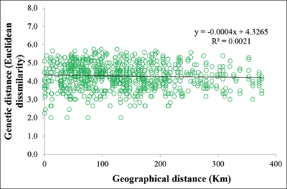
A mantel test was carried out to understand the correlation between the geographical and genetic distances of the Dalbergia species using GenAlEx software (version 6.502). The geographical distance was measured in Kilometers, whereas genetic distance was measured in Euclidean distance. The matrix table of geographical and genetic distances were created separately and used for this test [25].